Prediction of the landing distance of the Aircrafts

The purpose of this project is to solve a problem using linear regression and understand various feature selection and model selection techniques. In this project we predict the landing distance of the aircrafts based on different details. There have been many major mishaps during the landing of the aircraft, resulting in the loss of many lives. The data used in this project can be found here.

Information about various parameters such as, pitch, ground speed, air speed, height etc. of Airbus and Boeing aircrafts is given for the study.

We have to come up with a robust regression model that can predict the landing distance.

Packages Required

library(readxl)
library(ggplot2)
library(dplyr)
library(GGally)
library(leaps)
library(gridExtra)
library(plotly)
library(mvinfluence)
library(ggthemes)

Loading and cleaning the data

The data is stored in two excel sheets called FAA1 and FAA2 respectively. We need to load these sheets, analyse the data for completeness and then combine the two datasets into one.

str(faa1)

## Classes 'tbl_df', 'tbl' and 'data.frame':    800 obs. of  8 variables:
##  $ aircraft    : chr  "boeing" "boeing" "boeing" "boeing" ...
##  $ duration    : num  98.5 125.7 112 196.8 90.1 ...
##  $ no_pasg     : num  53 69 61 56 70 55 54 57 61 56 ...
##  $ speed_ground: num  107.9 101.7 71.1 85.8 59.9 ...
##  $ speed_air   : num  109 103 NA NA NA ...
##  $ height      : num  27.4 27.8 18.6 30.7 32.4 ...
##  $ pitch       : num  4.04 4.12 4.43 3.88 4.03 ...
##  $ distance    : num  3370 2988 1145 1664 1050 ...

str(faa2)

## Classes 'tbl_df', 'tbl' and 'data.frame':    150 obs. of  7 variables:
##  $ aircraft    : chr  "boeing" "boeing" "boeing" "boeing" ...
##  $ no_pasg     : num  53 69 61 56 70 55 54 57 61 56 ...
##  $ speed_ground: num  107.9 101.7 71.1 85.8 59.9 ...
##  $ speed_air   : num  109 103 NA NA NA ...
##  $ height      : num  27.4 27.8 18.6 30.7 32.4 ...
##  $ pitch       : num  4.04 4.12 4.43 3.88 4.03 ...
##  $ distance    : num  3370 2988 1145 1664 1050 ...

We can observe that the column duration is missing from FAA2 dataset. We need to introduce this column in order to merge two dataframes. We also check if we have any duplicate records in the combined dataframe.

# the column 'duration' is missing from faa2 dataframe
faa2$duration<-NA
# Now, we can concatinate the two dataframes
faa<-rbind(faa1,faa2)
str(faa)

## Classes 'tbl_df', 'tbl' and 'data.frame':    950 obs. of  8 variables:
##  $ aircraft    : chr  "boeing" "boeing" "boeing" "boeing" ...
##  $ duration    : num  98.5 125.7 112 196.8 90.1 ...
##  $ no_pasg     : num  53 69 61 56 70 55 54 57 61 56 ...
##  $ speed_ground: num  107.9 101.7 71.1 85.8 59.9 ...
##  $ speed_air   : num  109 103 NA NA NA ...
##  $ height      : num  27.4 27.8 18.6 30.7 32.4 ...
##  $ pitch       : num  4.04 4.12 4.43 3.88 4.03 ...
##  $ distance    : num  3370 2988 1145 1664 1050 ...

# Removing duplicates from the dataframe
dim(unique(faa))

## [1] 950   8

Removing outliers-

We have been given following information to decide whether an observation is an outlier or not:

The duration of a normal flight should always be greater than 40 min.
If Speed_ground is less than 30MPH or greater than 140MPH, then the landing would be considered as abnormal.
If Speed_air is less than 30MPH or greater than 140MPH, then the landing would be considered as abnormal.
The landing aircraft is required to be at least 6 meters high at the threshold of the runway.
Landing distance should be less than 6000 feet

Based on this information, we clean the dataset.

faa<-faa%>%filter(duration>40,speed_ground >= 30, speed_ground <=140,speed_air >= 30, speed_air <=140,height >=6,distance<6000)
summary(faa)

##    aircraft            duration        no_pasg       speed_ground   
##  Length:195         Min.   : 45.5   Min.   :41.00   Min.   : 88.69  
##  Class :character   1st Qu.:115.9   1st Qu.:56.00   1st Qu.: 95.28  
##  Mode  :character   Median :149.3   Median :60.00   Median :100.75  
##                     Mean   :150.9   Mean   :59.83   Mean   :103.43  
##                     3rd Qu.:185.4   3rd Qu.:65.00   3rd Qu.:109.57  
##                     Max.   :287.0   Max.   :80.00   Max.   :132.78  
##    speed_air          height           pitch          distance   
##  Min.   : 90.00   Min.   : 9.697   Min.   :2.702   Min.   :1741  
##  1st Qu.: 96.15   1st Qu.:23.365   1st Qu.:3.636   1st Qu.:2161  
##  Median :100.89   Median :29.837   Median :4.070   Median :2526  
##  Mean   :103.50   Mean   :30.359   Mean   :4.043   Mean   :2784  
##  3rd Qu.:109.42   3rd Qu.:36.590   3rd Qu.:4.442   3rd Qu.:3186  
##  Max.   :132.91   Max.   :58.228   Max.   :5.311   Max.   :5382

Once the data is cleaned, we sample 80% of the observation for training the regression model and the rest 20% for testing the model-

rows<-sample(195,0.8*195,replace = FALSE)
train<-faa[rows,]
test<-faa[-rows,]

# checking the correlation among variables
ggpairs(train)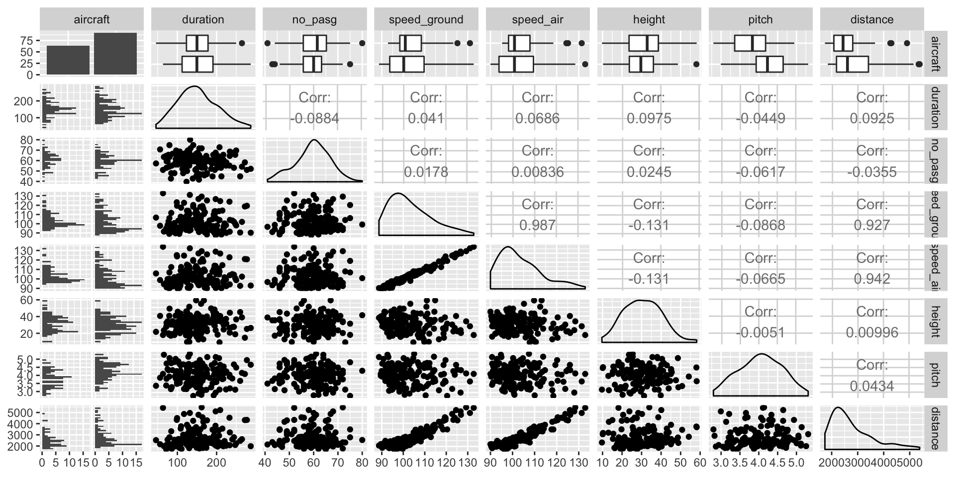

Since the dataset is small, we can use best subset selection for variable selection. Best subset selection algorithm will look for best subset of predictors that closely relate with the response variable. This method may not be best suited when the number of variables are too large.

We will use-

Adjusted R Squared
CP
BIC

As creterion for selecting the best subset of predictors for our linear model.

#Best subset variable selection
best.subset<-regsubsets(distance~.,data = train,nvmax = 7)
best.subset.summary <- summary(best.subset)

# Now, we will use different criterion to select the best subset of the predictors for our problem
# 1. Adjused R squared
p1<-ggplot(data = NULL,aes(x=1:7,y = best.subset.summary$adjr2))+geom_line(color='white')+labs(x='Index',y='Adjusted R Squared',title='Adjusted R Squared')+
  theme_hc(bgcolor = "darkunica")

# 2. CP
p2<-ggplot(data = NULL,aes(x=1:7,y = best.subset.summary$cp))+geom_line(color='white')+labs(x='Index',y='CP',title='CP')+
  theme_hc(bgcolor = "darkunica")

# 3. BIC
p3<-ggplot(data = NULL,aes(x=1:7,y = best.subset.summary$bic))+geom_line(color='white')+labs(x='Index',y='BIC',title='BIC')+
  theme_hc(bgcolor = "darkunica")

grid.arrange(p1,p2,p3)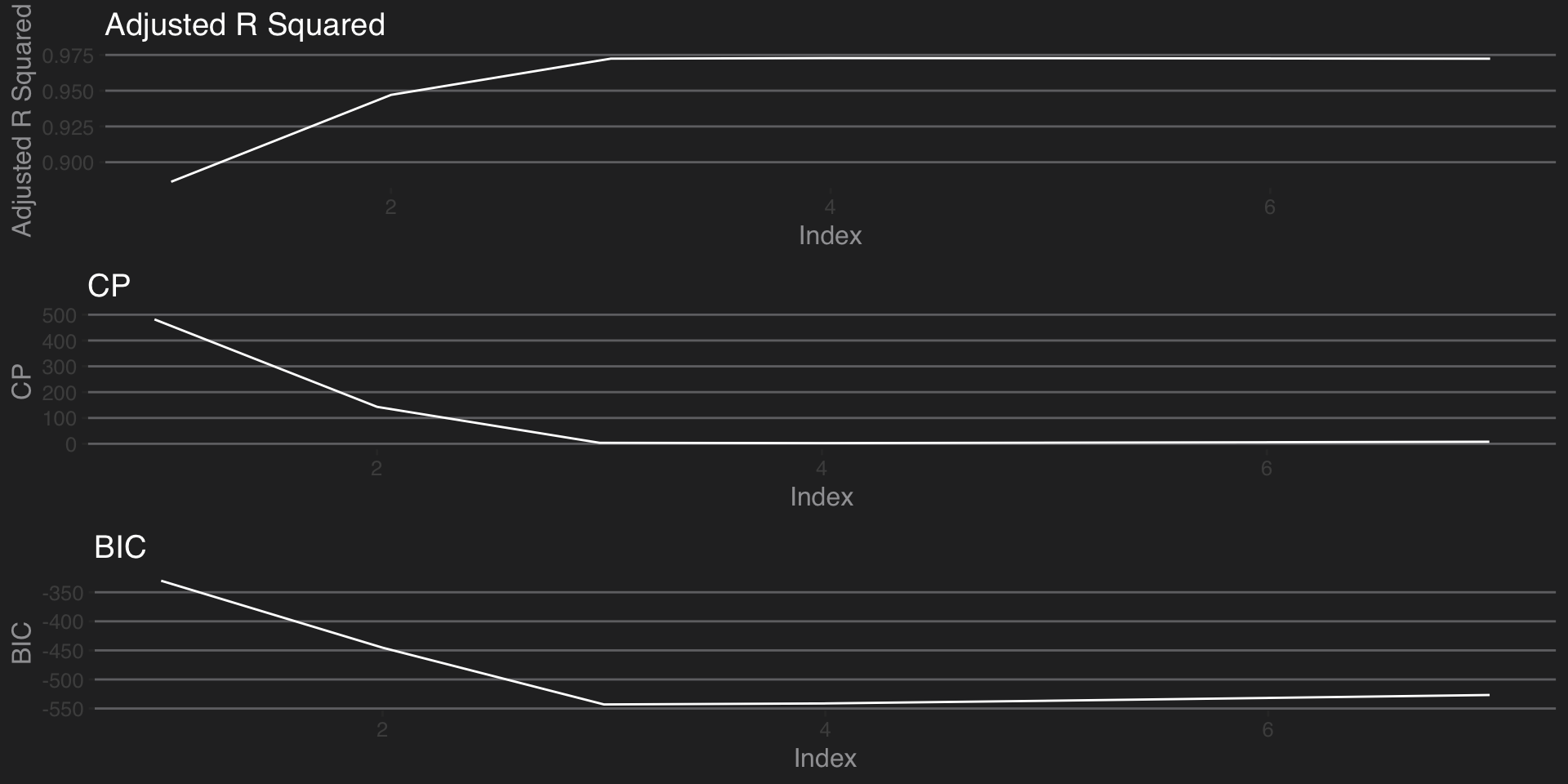

From above graphs, it is visible that-

Adjusted R Squared increases with index upto index 3, then almost stays constant
CP gets reduced with index up to 3, then almost stays constant
BIC reduces with index up to 3, later increases gradually

Thus,subset with index 3, is the best subset that leads to optimum results. We will use this subset for our linear model.

# The best model is model with index 3.
best.subset.summary$outmat[3,]

## aircraftboeing       duration        no_pasg   speed_ground      speed_air 
##            "*"            " "            " "            " "            "*" 
##         height          pitch 
##            "*"            " "

The best subset contains predictors- Aircraft, speed_air and height.

Before model the building, we try to visualise the relationship among the variables in a 3D graph just to get a sense of the data-

p <- plot_ly(train, x = ~speed_air, y = ~distance, z = ~height, color = ~aircraft, colors = c('red', 'blue'),alpha=0.5) %>%
  add_markers() %>%
  layout(scene = list(xaxis = list(title = 'Air Speed'),
                      yaxis = list(title = 'Landing Distance'),
                      zaxis = list(title = 'Height')))
p

Building the model-

We go ahead with building the model-

# Building linear regression model
model<-lm(data=train, distance~speed_air+aircraft+height)
summary(model)

## 
## Call:
## lm(formula = distance ~ speed_air + aircraft + height, data = train)
## 
## Residuals:
##     Min      1Q  Median      3Q     Max 
## -282.69 -100.70   19.50   92.79  343.84 
## 
## Coefficients:
##                 Estimate Std. Error t value Pr(>|t|)    
## (Intercept)    -6406.368    129.300  -49.55   <2e-16 ***
## speed_air         82.128      1.136   72.30   <2e-16 ***
## aircraftboeing   434.082     22.230   19.53   <2e-16 ***
## height            13.659      1.148   11.90   <2e-16 ***
## ---
## Signif. codes:  0 '***' 0.001 '**' 0.01 '*' 0.05 '.' 0.1 ' ' 1
## 
## Residual standard error: 135.8 on 152 degrees of freedom
## Multiple R-squared:  0.973,  Adjusted R-squared:  0.9724 
## F-statistic:  1823 on 3 and 152 DF,  p-value: < 2.2e-16

Model Diagnostics

par(mfrow=c(2,2))
plot(model)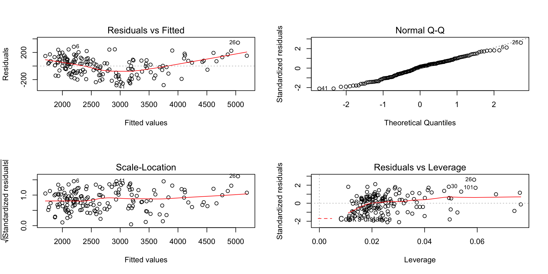

par(mfrow=c(1,1))
infIndexPlot(model, var="cook", main="Index Influence Plot")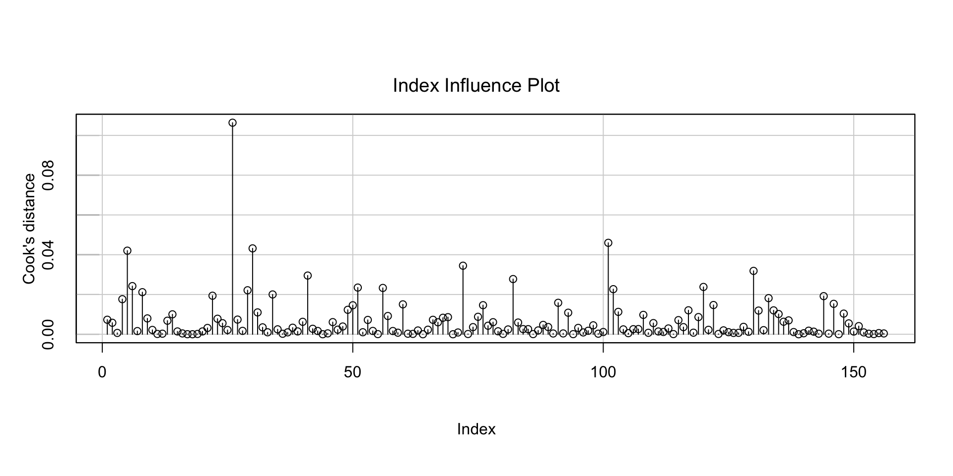

From the graphs we can see that- * The residuals are normally distributed (Q-Q plot) * The residuals have constant variance * There are no obvious high laverage or high influence points

Observation with index 6, has high Cook’s Distance, 0.11. Let’s take a closer look at this observation-

# point has high Studentized Residual > 2 but < 3
a<-as.numeric(train[6,5])
b<-as.numeric(train[6,8])
ggplot(data = train,aes(x = speed_air,y = distance,color=aircraft))+geom_point()+geom_smooth(method='lm')+
  geom_point(aes(x=a,y=b),color='Purple')+annotate("text", x = 125, y = 5400, label = "Possible Outlier",col='Purple')+
  theme_hc(bgcolor = "darkunica")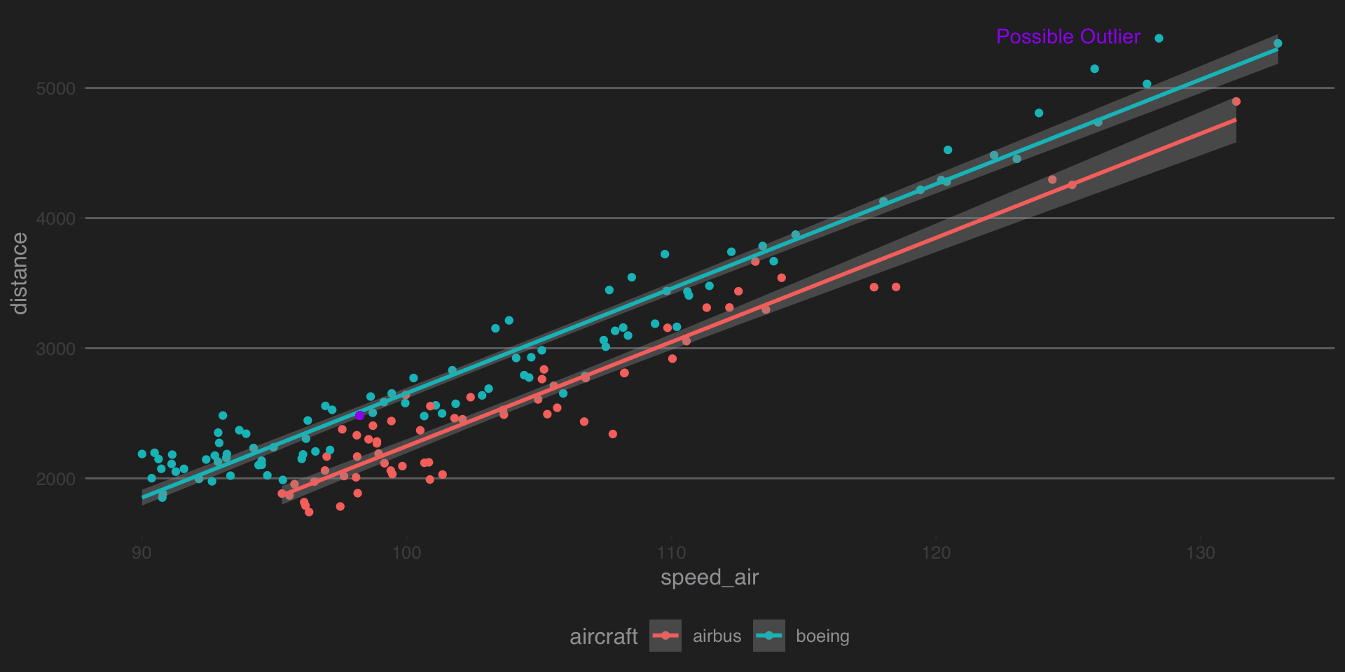

influencePlot(model)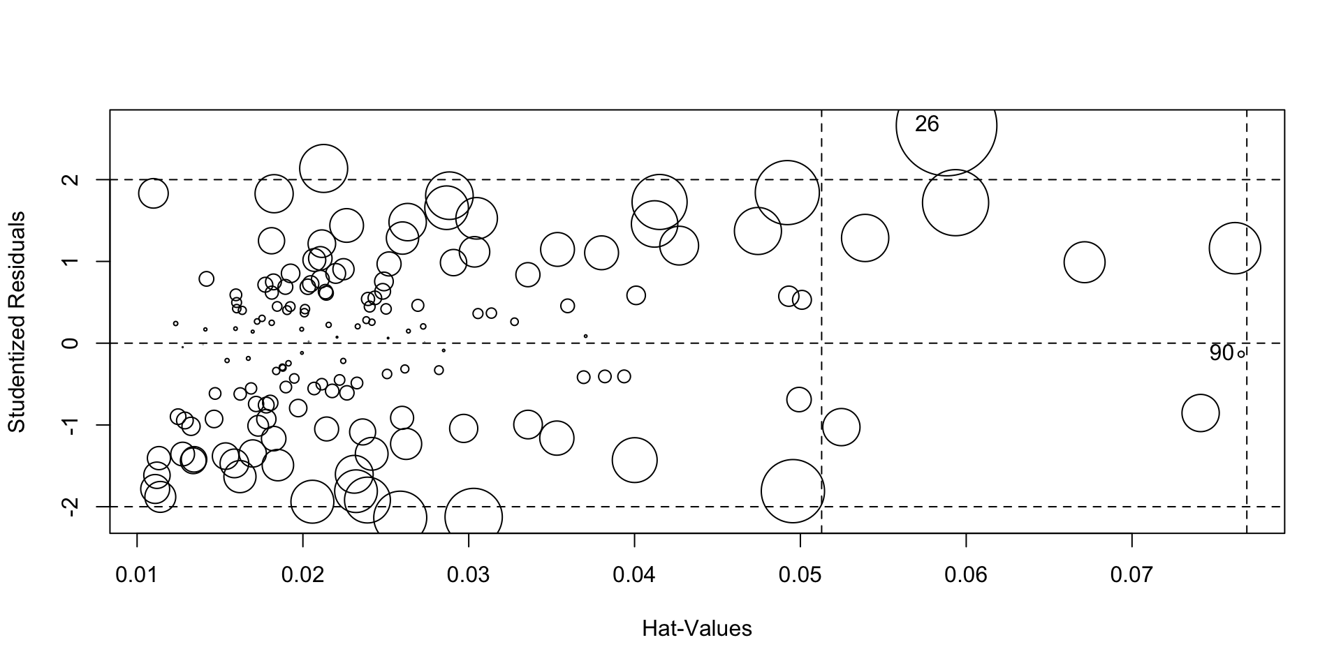

##       StudRes        Hat        CookD
## 26  2.6613084 0.05881641 0.1063932807
## 90 -0.1349164 0.07658111 0.0003798453

However, the Studentized Residual for that observation is less than 3. Thus, we will not consider that point to be an outlier.

Prediction on the Test data-

Now we try to predict the landing distance of the observations from test data.

test$predictedDistance<-predict(model,test)
cor.test(test$distance,test$predictedDistance)

## 
##  Pearson's product-moment correlation
## 
## data:  test$distance and test$predictedDistance
## t = 46.015, df = 37, p-value < 2.2e-16
## alternative hypothesis: true correlation is not equal to 0
## 95 percent confidence interval:
##  0.9834906 0.9955034
## sample estimates:
##       cor 
## 0.9913758

ggplot(data = test,aes(distance,y=predictedDistance,color=aircraft))+geom_point()+labs(x='Actual Distance',
      y='Predicted Distance',title='Prediction Graph')+theme_hc(bgcolor = "darkunica")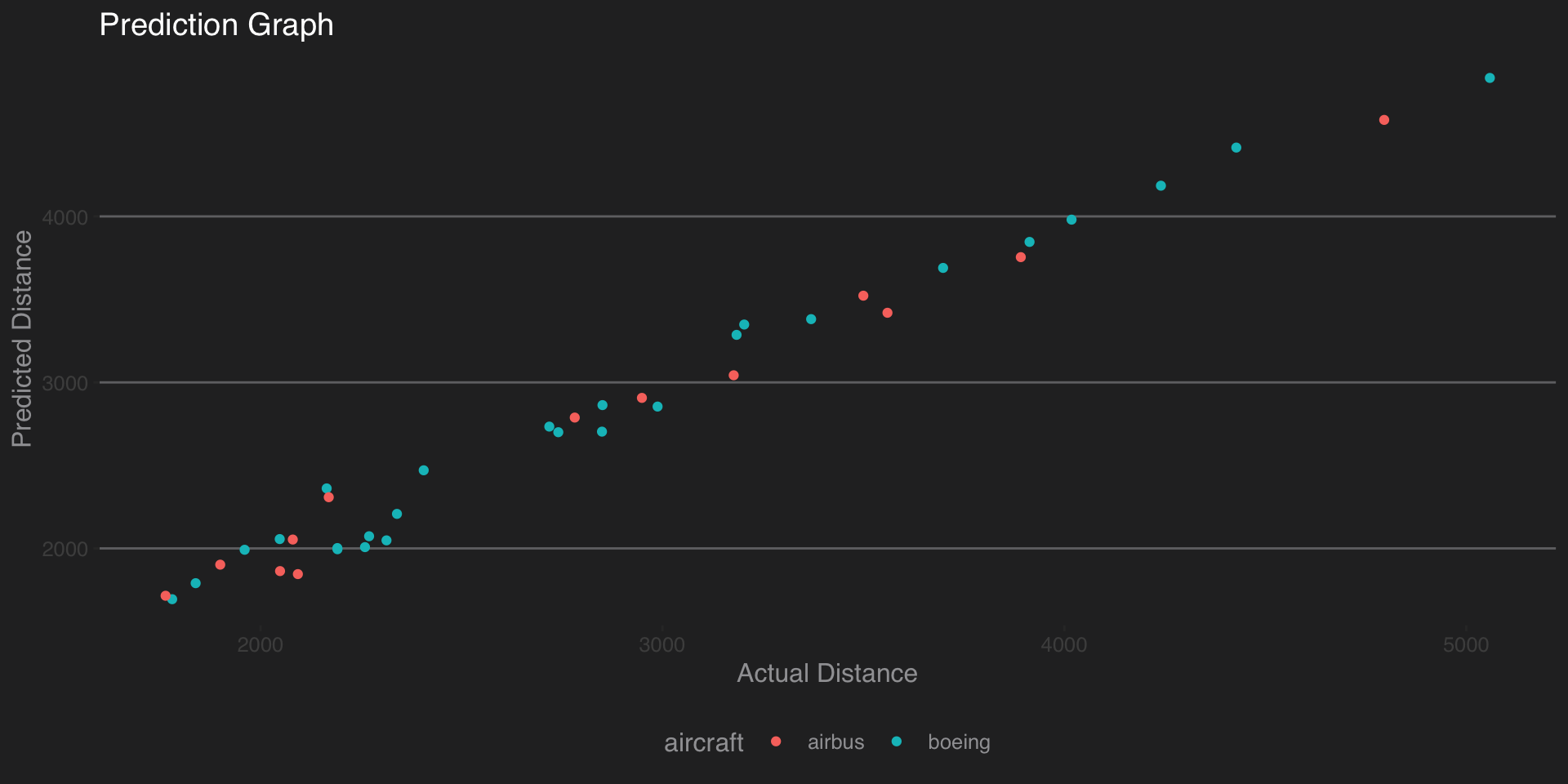

We can se that the correlation coefficient between actual landing distance and the predicted landing distance is 0.9891462 with 95% Confidence Interval being 0.9792438, 0.9943379. The prediction is fairly accurate as it predicts with close to 98% accuracy.

Thus, we can say that the Liner Regression model does a good job of predicting the landing distance.

Predicting Landing Distance of Aircraft